Why Does Pi Show up in the Normal Distribution?

06 Dec 2021

While recently looking through an old stats textbook, I came across the familiar equation for the normal distribution:

\[ f(x) = \frac{1}{\sigma\sqrt{2\pi}}e^{-\frac{1}{2}(\frac{x-\mu}{\sigma})^{2}} \]

Anyone that’s taken a statistics course in university has come across this equation. I had seen it many times myself, but looking at it fresh this time, two questions immediately came to mind:

1. How exactly does this thing form a normal distribution?
2. What the hell is \( \pi \) doing in there?

The first question seemed simple enough to figure out: I would just have to trace back the history of the equation and put it together piece by piece. But the second question absolutely stumped me: what in the world does a bell curve have to do with a circle?

I read through all of the Math Stackexchange solutions, searched around, and asked on Twitter, but never felt like any of the answers gave me the intuition I was looking for. They relied too heavily on analytical solutions, or when visual techniques were employed, the connections felt hand-wavy to me. After doing a bit of my own research, here’s my attempt at explaining the connection without resorting to any advanced math.

First, what exactly is a bell curve?

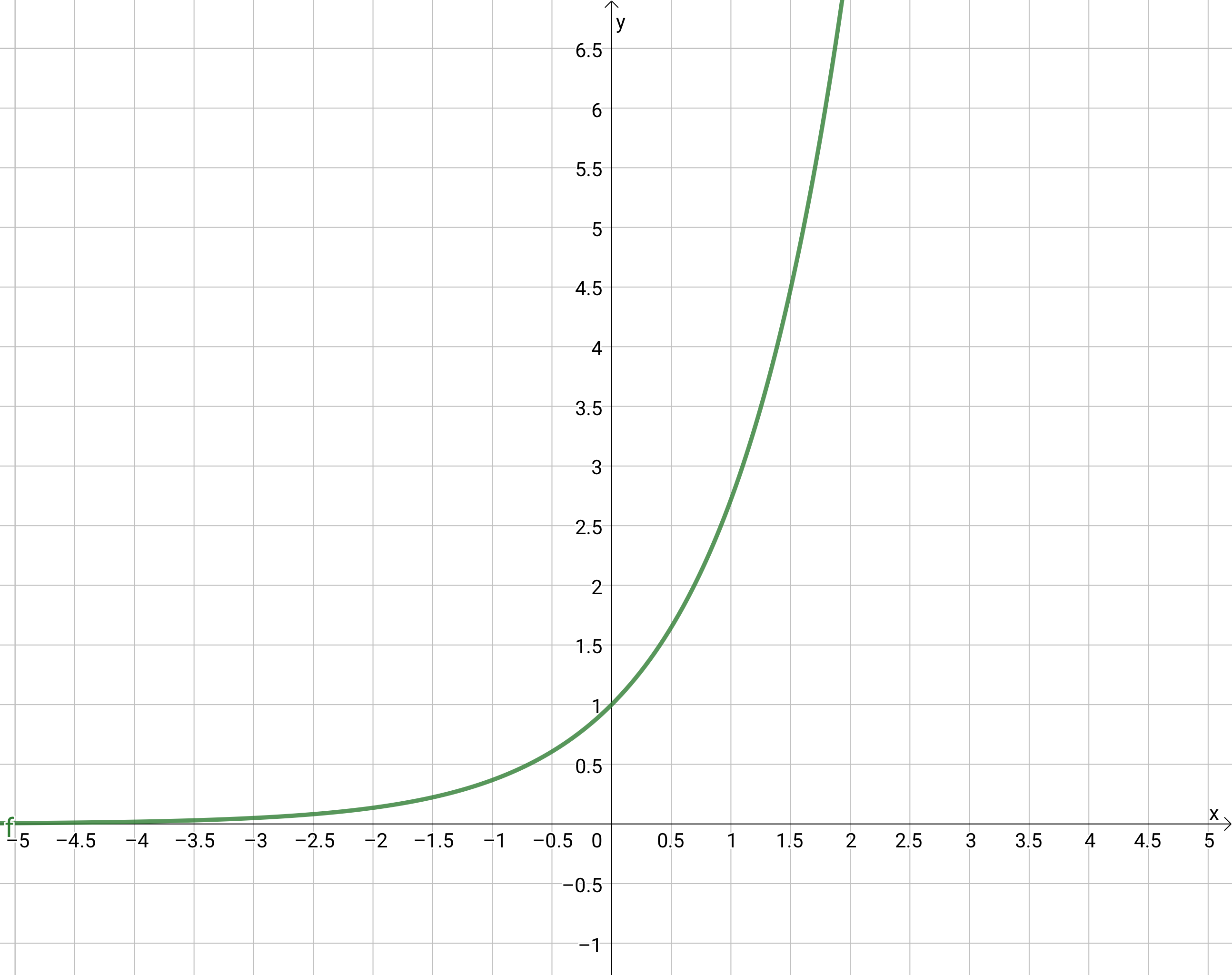
Before we get to the \( \pi \) part, it helps to gain some insight into how exactly a bell curve is formed. Let’s start with the exponential function, which you can see within the equation above. Here it is standing on its own:

\[ f(x) = e^{x} \]

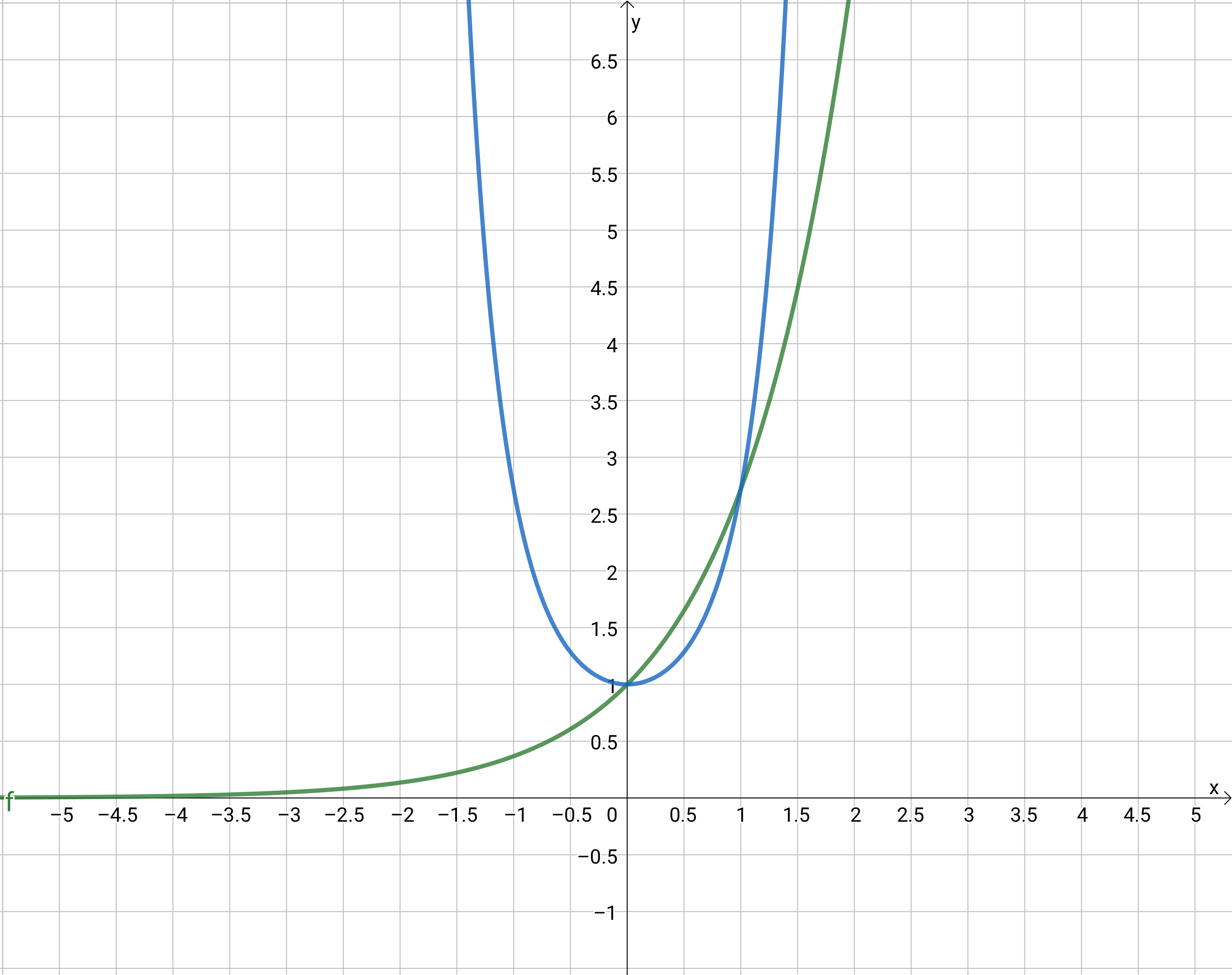
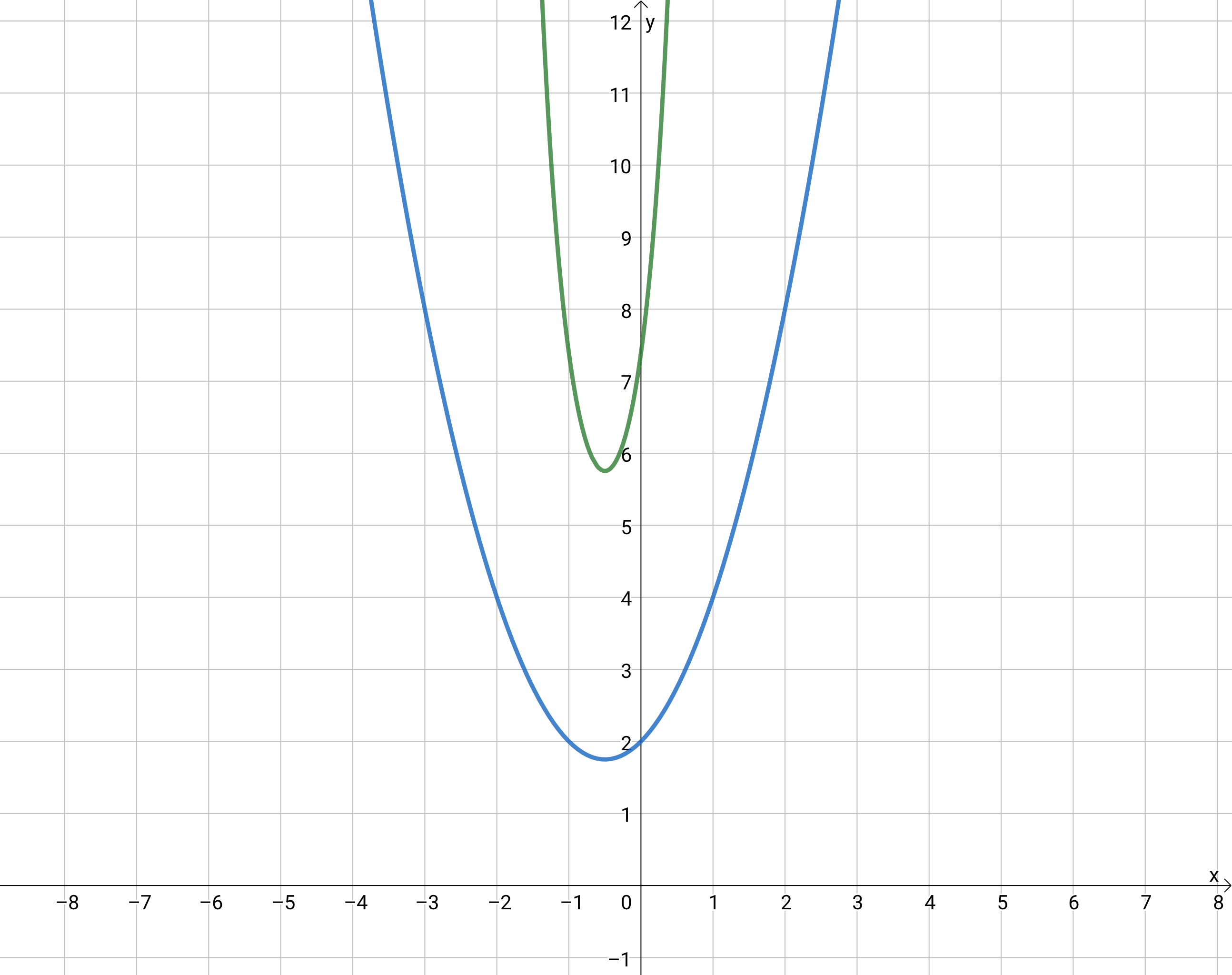
If we square the value of \( x \), it turns into something that looks kind of like a quadratic, but isn’t one. Instead, it’s a function that grows much faster than a quadratic, but has some similar properties such as being symmetric about its lowest point. Adding it to the plot above for comparison, you can see that they have the same value at \( x=0 \) and \( x=1 \):

\[ f(x) = e^{x^2} \]

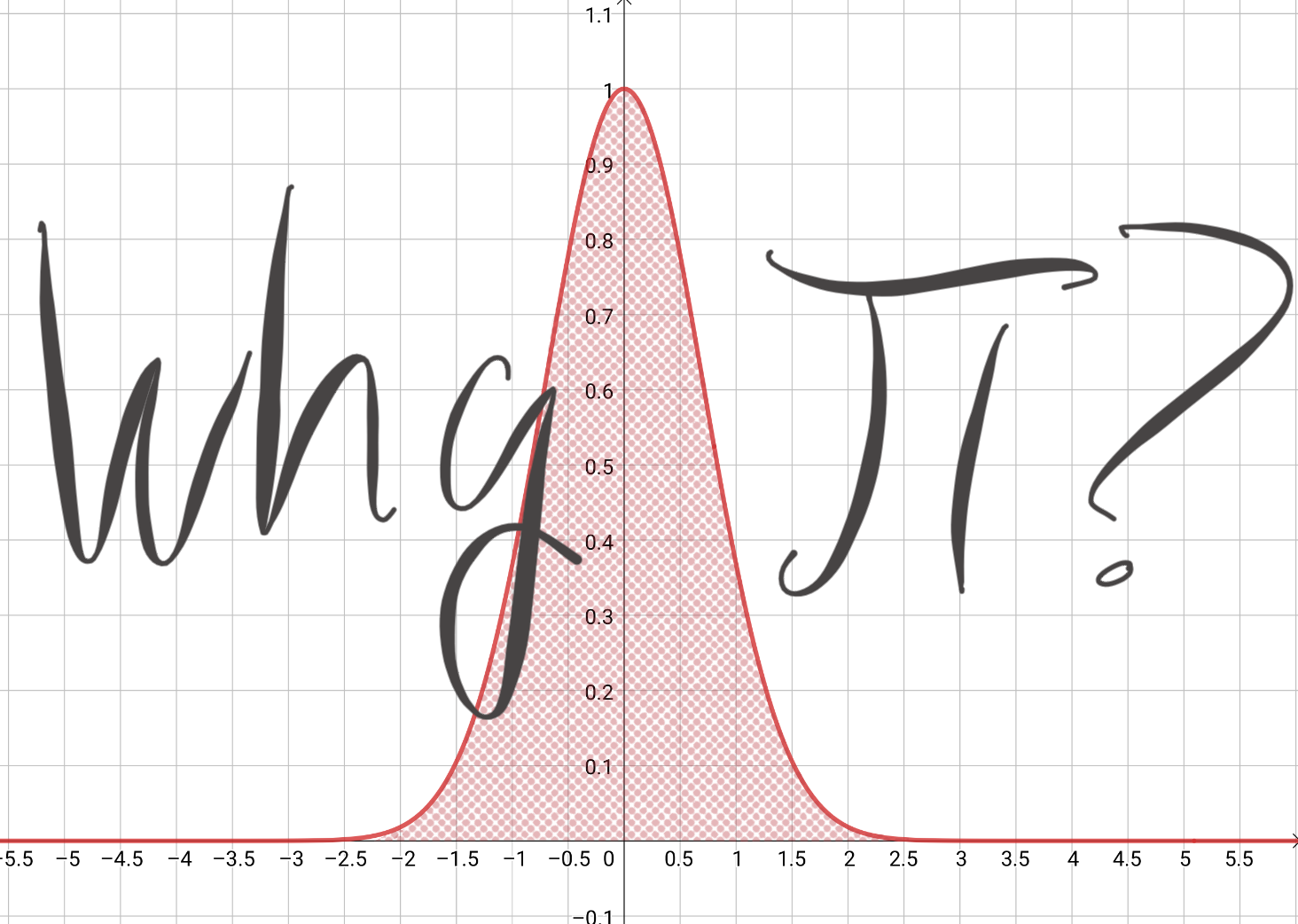
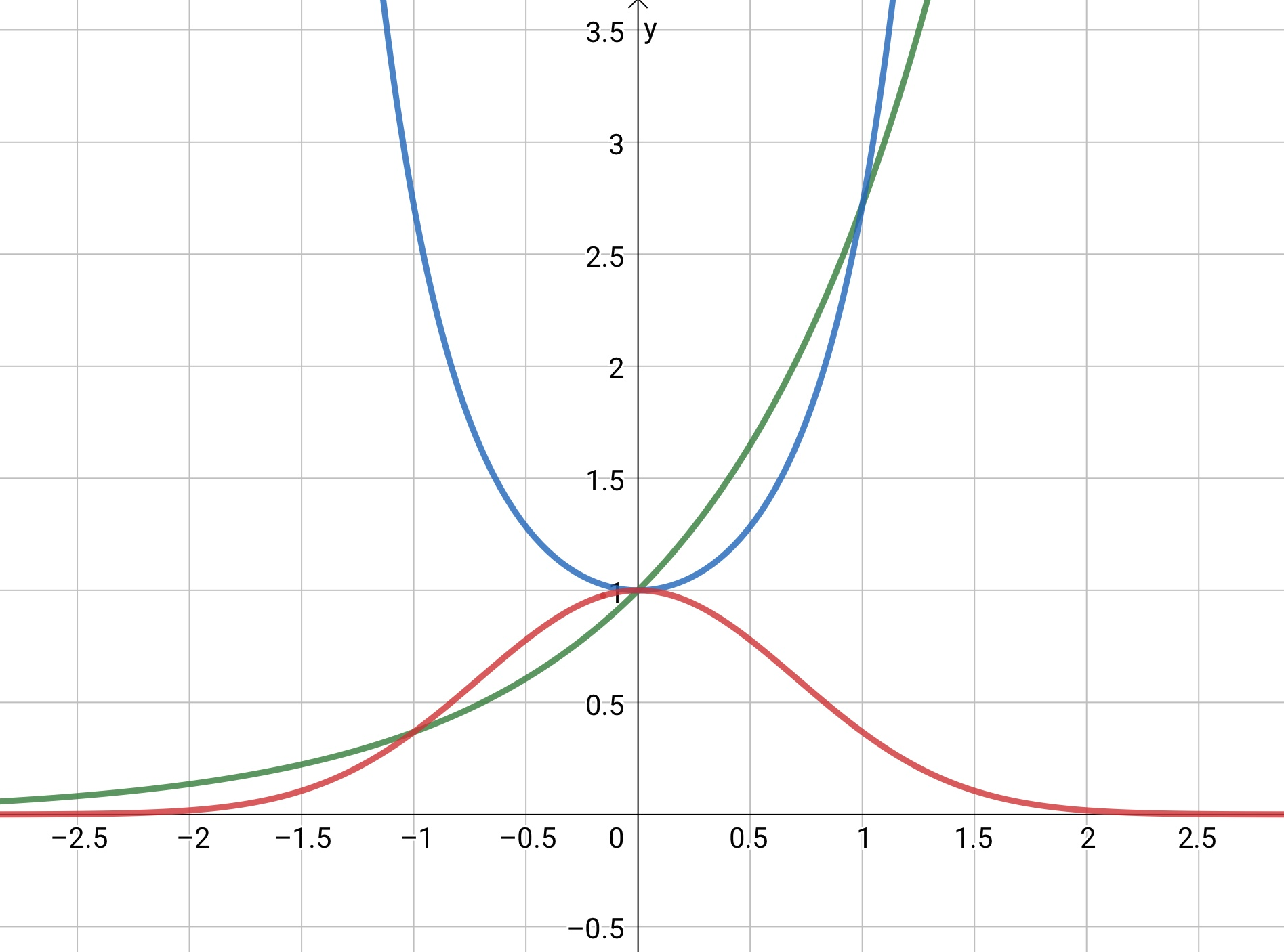
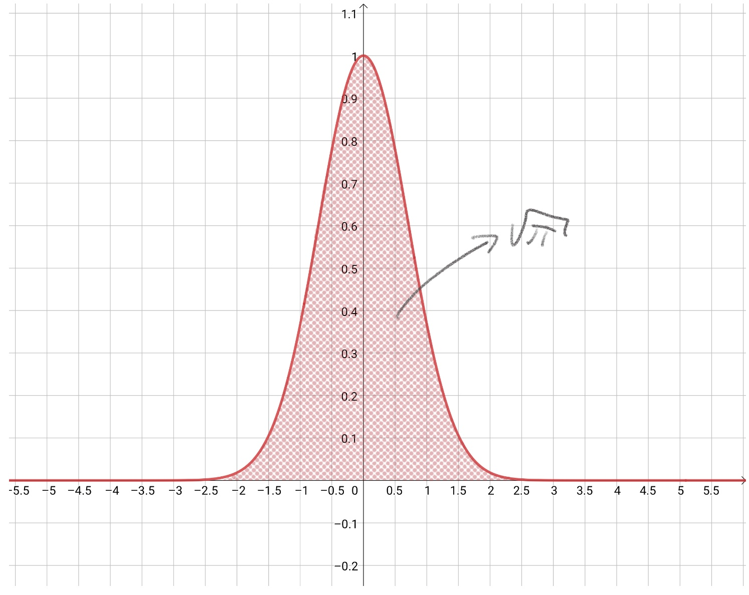
Finally, let’s make the exponent negative, and like magic, we get the bell curve shown in red below:

\[ f(x) = e^{-x^2} \]

This function, \( f(x) = e^{-x^2} \), is just one particular bell curve of an infinite number of possibilities. In general, you can raise \( e \) to any quadratic you like. However, it is only when that quadratic is concave (that is, it “opens” downwards) that you get a bell curve. Above, that quadratic was \( -x^2 \), which does indeed open downwards.

For example, the equation \( f(x) = x^2 + x + 2 \) plotted in blue below is not concave, and when \( e \) is raised to it, you get the green curve, which is obviously not a bell curve:

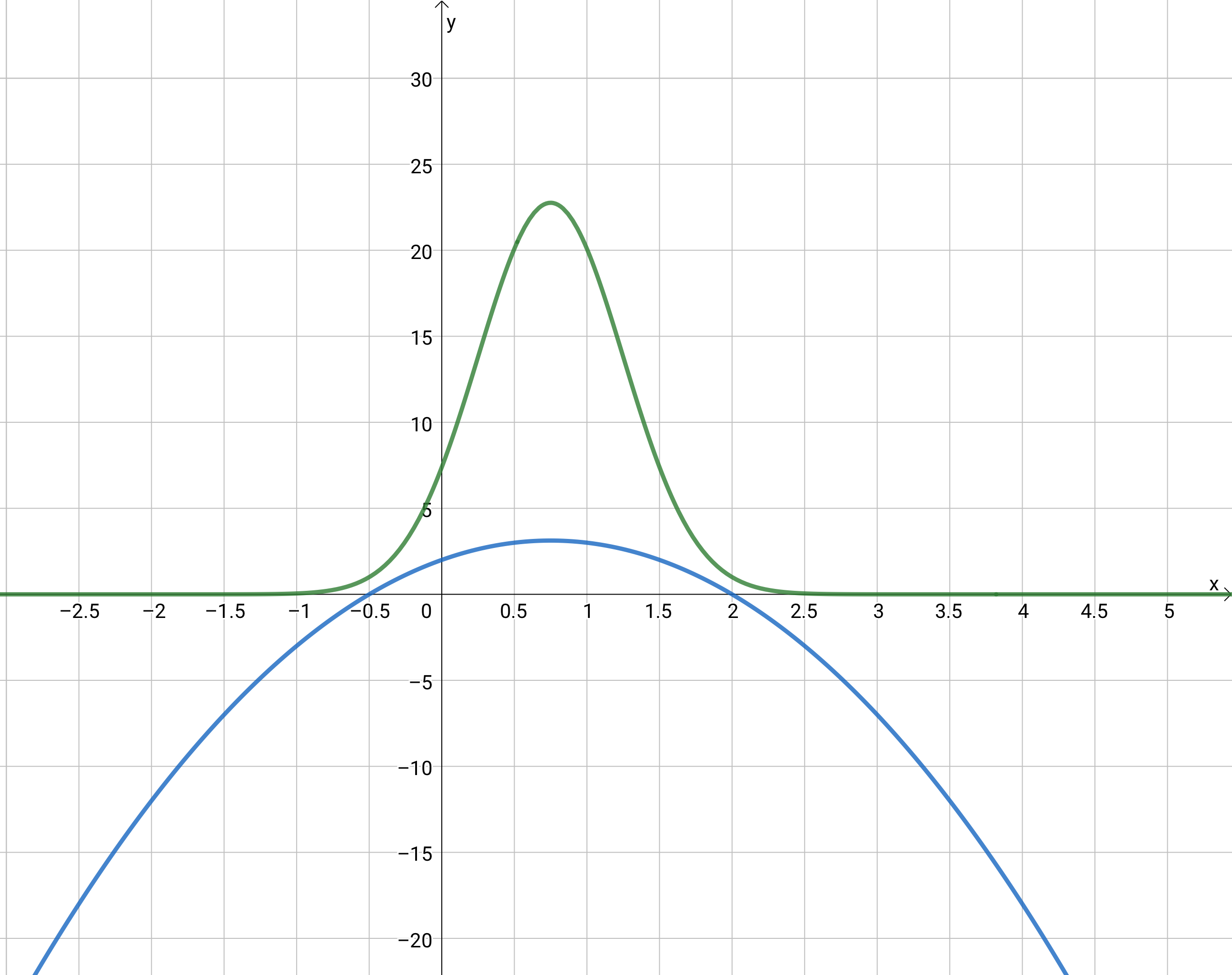
If we switch the equation to be \( f(x) = -2x^2 + 3x + 2 \), though, we get a concave function, and \( e \) raised to that forms the bell curve shape:

For this reason, the general equation of a equation of a bell curve is \( e \) raised to a quadratic:

\[ f(x) = e^{\alpha x^2 + \beta x + \gamma} \]

To help constrain it to only concave quadratics, you can perform the following replacements:

\[ \alpha = \frac{-1}{2\sigma^{2}} \] \[ \beta = \frac{\mu}{\sigma^{2}} \] \[ \gamma = \ln(a) - \frac{\mu^2}{2\sigma^2} \]

After you substitue these in and rearrange, you’ll find that you get the following, which is almost exactly the equation we started with at the top, only with an \( a \) in front of it:

\[ f(x) = ae^{-\frac{1}{2}(\frac{x-\mu}{\sigma})^{2}} \textbf{ vs } f(x) = \frac{1}{\sigma\sqrt{2\pi}}e^{-\frac{1}{2}(\frac{x-\mu}{\sigma})^{2}} \]

The \( a \) is chosen in the equation on the right so that no matter what shape the bell curve takes, the area underneath it is always exactly 1. This is because for a statistical distribution, 1 is equivalent to 100% of the possible outcomes, and the area should always sum to that value.

So, in other words, the connection between the bell curve and that \( \pi \) term must have something to do with the area of the curve itself. But what exactly is that connection?

How Pi is related to the bell curve

Before I get to how \( \pi \) is related, let me first state a fact and let you chew on it for a moment: if we return to one of the equations above, \( f(x) = e^{-x^2} \), it turns out that the area under this curve is exactly \( \sqrt{\pi}\).

Let’s take stock of what just happened there. We took a transcendental number, \( e \), and raised it to the power of a quadratic. When we calculate the area under that curve, we get another transcendental number, Pi.

It turns out that these two numbers are related in a few ways, including their relationship in the complex number system via one of the most beautiful equations in math: \( e^{i\pi} + 1 = 0 \). But that equation doesn’t play a role here.

Instead, as we’ll see, \( \pi \) comes out of the way that we have to go about calculating the area. In a roundabout way, we can get this area by working with the square of \( e^{-x^2} \), and then taking the square root. In other words:

\[ \sqrt{( \text{Area of } e^{-x^2})\cdot (\text{Area of } e^{-x^2})} \]

The reason we have to do this has to do with the calculus technique that we need to employ to get the area. There’s plenty of examples online that show how to do this, but I want to instead provide the visual intuition that these analytic solutions don’t necessarily convey.

Since the variable we use to calculate the area is arbitrary, we can just as easily represent the above equation as the following, where we replaced the second \( x \) with a \( y \):

\[ \sqrt{( \text{Area of } e^{-x^2})\cdot (\text{Area of } e^{-y^2})} \]

You can now think of this as putting one of these bell curves on the x-axis and the other on the y-axis, and then getting all combinations of their heights and plotting it in 3 dimensions:

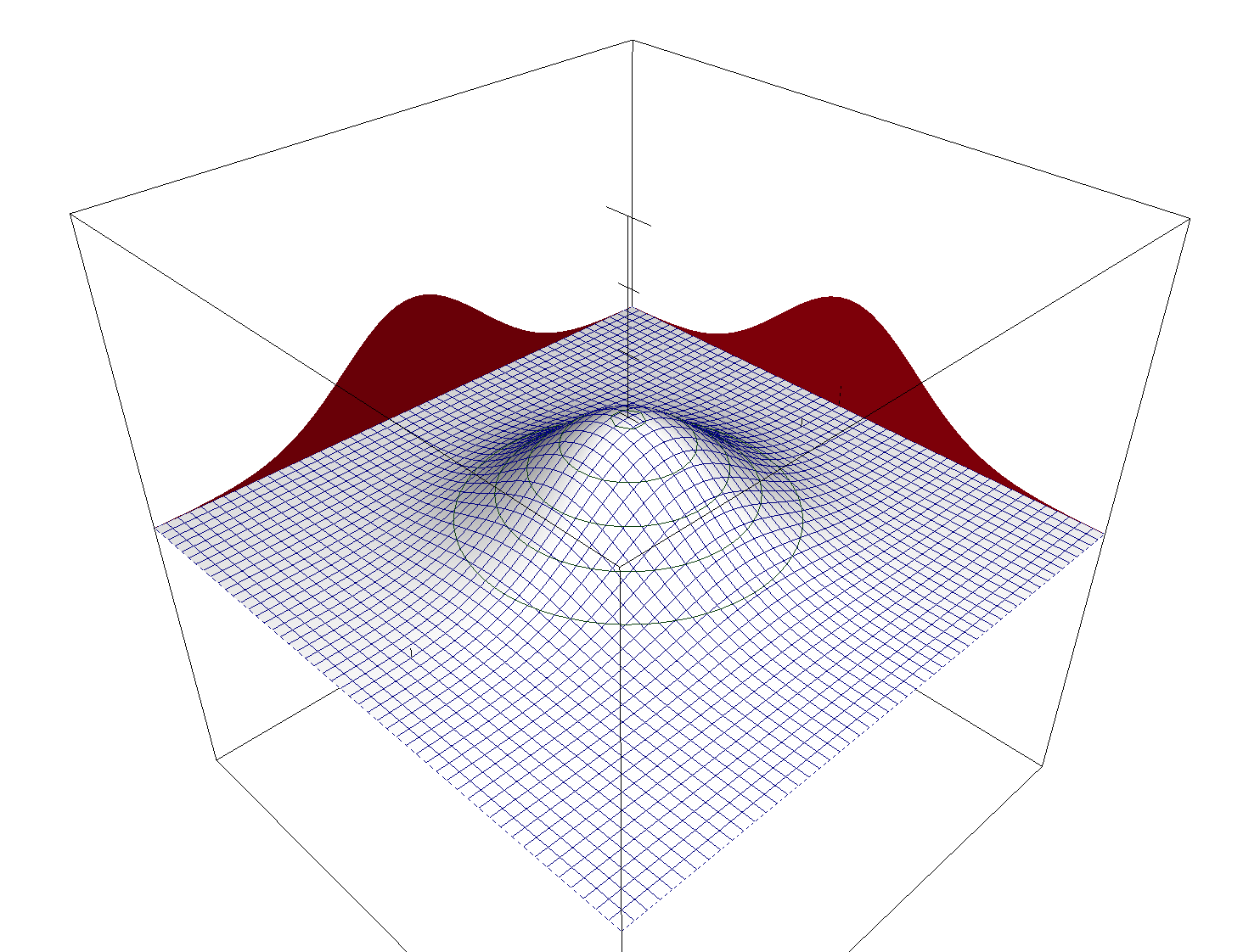
To get the area of one of the curves, you just need to get the volume of the “hill” that forms, and then take the square root of that value. An analogy to this with fewer dimensions is knowing the area of a square, and then getting its side length by taking the square root.

Note: This trick will not work for all types of functions. If you try this with a quadratic (say, \( -x^2 + 9 \)), you will not get the correct answer. The reason is that this only works for functions that are rotationally symmetric when they are squared. While the Gaussian is, you can see from a similar plot of the quadratic that it is "boxy" and is not symmetric through rotation the way that the curve above is:

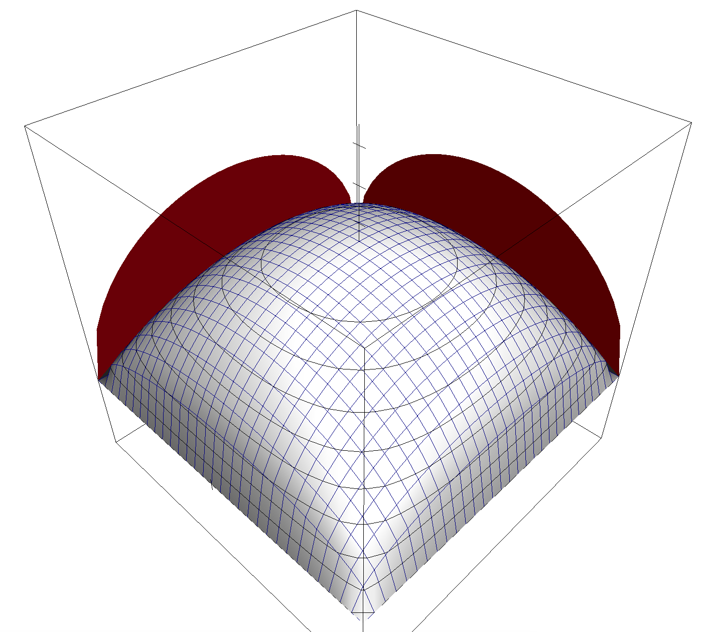
OK, so how do we get the volume of the “hill” above? One way would be to chunk it up into squares like above, and then get the height of each in the middle of the square. You could then calculate the volume of these square pillars as \( (\text{Area of Each Square}) \cdot (\text{Height}) \) and then add up all those smaller volumes. The smaller you make the squares, the better the approximation.

However, this hides where the \( \pi \) comes from. So instead, imagine that instead of using squares, we divide it up radially. In this diagram, we are looking down from the top and we see the contour lines of the hill:

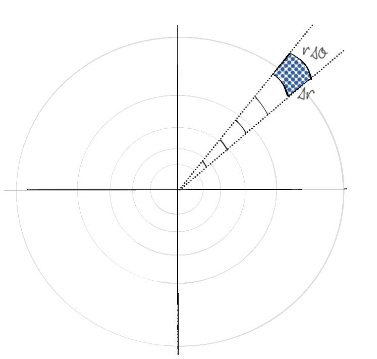
Here, you divide up the hill into “slices” represented by the black dotted lines. Those slices are further divided into pieces as highlighted in blue. As above, you multiply the area of each of these blue pieces by the height of the hill at that point to get the volume.

\[ r \Delta \theta \Delta r \cdot \text{Height} \]

In this case, though, you repeat this along the “slice” to get the volume of the entire slice, and then multiply that by the total number of slices to get the entire volume of the hill.

If you make the angle \( \theta \) small enough so that it’s barely a sliver, then for all intents and purposes, you can multiply the volume of a slice by \( 2 \pi \text{ radians}\), the number of radians in a circle.

If you actually do this math (again, the calculus is covered here for those that want to see it in action) you’ll find that each slice has an area of exactly \( \frac{1}{2} \). Multiplying that by \( 2 \pi \text{ radians}\) and you get a volume that exactly equals \( \pi \).

So there you have it: \( \pi \) comes out of the fact that we find the volume by making radial slices, and then stitching them all together around a circle.

As it turns out, anything that is symmetric through rotation can be thought of as involving circles, and naturally, circles imply that \( \pi \) is lurking somewhere in the math.

While this isn’t a rigorous proof and I skipped over a lot of details (e.g. the jump to the 3D plot of the two bell curves doesn’t generally work for all functions, but it does for the ones we used) I hope that this gives readers an intuition for why \( \pi \) seems to show up out of nowhere in a curve that has seemingly little to do with it.